library(rfintext)
# devtools::install_github("StranMax/rfinstats")
library(rfinstats)
library(tidymodels)
library(topicmodels)
library(cowplot)
library(dplyr)
library(tidytext)
library(ggplot2)
library(quanteda)
library(forcats)
library(purrr)
library(future)  # Parallel processing back-end
library(furrr)  # Parallel processing front-end with future_ functions
plan(multisession, workers = availableCores(logical = FALSE) - 1)
dtm <- aspol |>
  preprocess_corpus(kunta) |>
  corpus_to_dtm(kunta, LEMMA)
y <- rfinstats::taantuvat |>
  filter(kunta %in% unique(aspol$kunta)) |>
  mutate(luokka = if_else(suht_muutos_2010_2022 > 0, "kasvava", "taantuva"))
y
#> # A tibble: 66 × 5
#>    kunta       vaesto kokmuutos_2010_2022 suht_muutos_2010_2022 luokka
#>    <chr>        <int>               <int>                 <dbl> <chr>
#>  1 Enontekiö     1876                 -71                 -3.78 taantuva
#>  2 Espoo       247970               60944                 24.6  kasvava
#>  3 Eura         12507               -1278                -10.2  taantuva
#>  4 Hartola       3355                -814                -24.3  taantuva
#>  5 Hattula       9657                -266                 -2.75 taantuva
#>  6 Helsinki    588549               80678                 13.7  kasvava
#>  7 Huittinen    10663                -955                 -8.96 taantuva
#>  8 Hyvinkää     45489                1527                  3.36 kasvava
#>  9 Hämeenlinna  66829                1588                  2.38 kasvava
#> 10 Iitti         7005                -557                 -7.95 taantuva
#> # ℹ 56 more rows
optimal_params <- lda_models |>
  filter(K == 18) |>
  slice_max(mean_coherence, n = 1)
optimal_params
#> # A tibble: 1 × 3
#>       K       S mean_coherence
#>   <int>   <int>          <dbl>
#> 1    18 5883911          -9.39
# optimal_k <- c(5, 15, 18, 21)
# optimal_k <- c(5, 8, 11, 14, 19)
# optimal_k <- c(5, 7, 10, 15, 21)  # Visually selected based on mean topic coherence (see article 3)
ptm <- proc.time()
lda_models <- optimal_params |>
  # slice_max(mean_coherence, n = 1) |>
  mutate(
    # LDA model
    topic_model = future_map2(
      K, S, \(k, s) {
        LDA(dtm, k = k, control = list(seed = S))
      }, .options = furrr_options(seed = NULL)
    ),
    # Beta matrix
    beta = map(
      topic_model, \(x) tidy(x, matrix = "beta")
    ),
    # Theta matrix (gamma)
    theta = map(
      topic_model, \(x) {
        tidy(x, matrix = "gamma") |>
          filter(document %in% y$kunta) |>
          rename(kunta = document, theta = gamma)
      }
    )
  )
proc.time() - ptm
#>    user  system elapsed
#>   1.166   0.047  45.084
lda_models
#> # A tibble: 1 × 6
#>       K       S mean_coherence topic_model beta                  theta
#>   <int>   <int>          <dbl> <list>      <list>                <list>
#> 1    18 5883911          -9.39 <LDA_VEM>   <tibble [54,684 × 3]> <tibble>
lda_models <- lda_models |>
  mutate(theta = map(theta, \(df) {
    df |>
      left_join(y) |>
      select(aihe = topic, theta, luokka) |>
      mutate(luokka = factor(luokka))
  }))
#> Joining with `by = join_by(kunta)`
lda_models
#> # A tibble: 1 × 6
#>       K       S mean_coherence topic_model beta                  theta
#>   <int>   <int>          <dbl> <list>      <list>                <list>
#> 1    18 5883911          -9.39 <LDA_VEM>   <tibble [54,684 × 3]> <tibble>
We calculate null distribution of t-values and observed t-value:
ptm <- proc.time()
t_distributions <- lda_models |>
  select(K, theta) |>
  unnest(theta) |>
  nest(data = c(theta, luokka)) |>
  mutate(
    null_dist = future_map(data, \(df) {
      # t-distribution under null hypothesis
      df |>
        specify(theta ~ luokka) |>
        hypothesize(null = "independence") |>
        generate(reps = 100000, type = "permute") |>
        calculate("diff in means", order = c("kasvava", "taantuva"))
    }, .options = furrr_options(seed = TRUE)),
    # t-value for estimation
    t_val = map_dbl(data, \(df) {
      df |>
        specify(theta ~ luokka) |>
        calculate("diff in means", order = c("kasvava", "taantuva")) |>
        pull(stat)
    })
  )
proc.time() - ptm
#>    user  system elapsed
#>   9.044   0.218 164.645
t_distributions
#> # A tibble: 18 × 5
#>        K  aihe data              null_dist                t_val
#>    <int> <int> <list>            <list>                   <dbl>
#>  1    18     1 <tibble [66 × 2]> <infer [100,000 × 2]>  0.0443
#>  2    18     2 <tibble [66 × 2]> <infer [100,000 × 2]> -0.107
#>  3    18     3 <tibble [66 × 2]> <infer [100,000 × 2]> -0.0524
#>  4    18     4 <tibble [66 × 2]> <infer [100,000 × 2]> -0.0456
#>  5    18     5 <tibble [66 × 2]> <infer [100,000 × 2]> -0.285
#>  6    18     6 <tibble [66 × 2]> <infer [100,000 × 2]>  0.00608
#>  7    18     7 <tibble [66 × 2]> <infer [100,000 × 2]>  0.0424
#>  8    18     8 <tibble [66 × 2]> <infer [100,000 × 2]> -0.00678
#>  9    18     9 <tibble [66 × 2]> <infer [100,000 × 2]>  0.135
#> 10    18    10 <tibble [66 × 2]> <infer [100,000 × 2]>  0.0232
#> 11    18    11 <tibble [66 × 2]> <infer [100,000 × 2]>  0.0585
#> 12    18    12 <tibble [66 × 2]> <infer [100,000 × 2]> -0.0400
#> 13    18    13 <tibble [66 × 2]> <infer [100,000 × 2]>  0.0117
#> 14    18    14 <tibble [66 × 2]> <infer [100,000 × 2]>  0.130
#> 15    18    15 <tibble [66 × 2]> <infer [100,000 × 2]>  0.0173
#> 16    18    16 <tibble [66 × 2]> <infer [100,000 × 2]> -0.0809
#> 17    18    17 <tibble [66 × 2]> <infer [100,000 × 2]>  0.0663
#> 18    18    18 <tibble [66 × 2]> <infer [100,000 × 2]>  0.0819
Next we calculate p-values:
t_distributions <- t_distributions |>
mutate(
p_value = pmap_dbl(select(t_distributions, null_dist, t_val), \(null_dist, t_val) {
null_dist |>
get_p_value(obs_stat = t_val, direction = "two-sided") |>
pull(p_value)
})
)
t_distributions
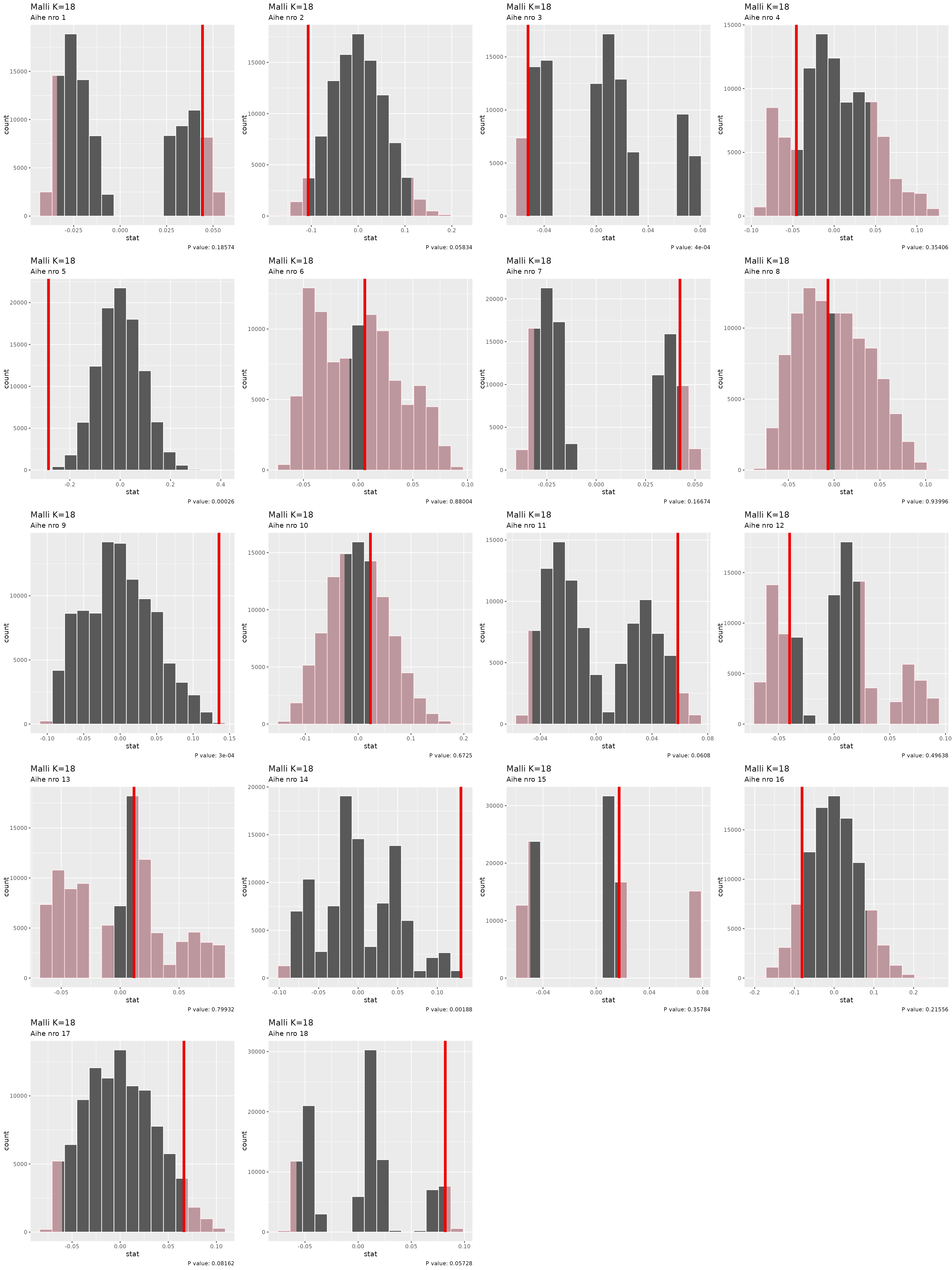
#> # A tibble: 18 × 6
#> K aihe data null_dist t_val p_value
#> <int> <int> <list> <list> <dbl> <dbl>
#> 1 18 1 <tibble [66 × 2]> <infer [100,000 × 2]> 0.0443 0.186
#> 2 18 2 <tibble [66 × 2]> <infer [100,000 × 2]> -0.107 0.0583
#> 3 18 3 <tibble [66 × 2]> <infer [100,000 × 2]> -0.0524 0.0004
#> 4 18 4 <tibble [66 × 2]> <infer [100,000 × 2]> -0.0456 0.354
#> 5 18 5 <tibble [66 × 2]> <infer [100,000 × 2]> -0.285 0.00026
#> 6 18 6 <tibble [66 × 2]> <infer [100,000 × 2]> 0.00608 0.880
#> 7 18 7 <tibble [66 × 2]> <infer [100,000 × 2]> 0.0424 0.167
#> 8 18 8 <tibble [66 × 2]> <infer [100,000 × 2]> -0.00678 0.940
#> 9 18 9 <tibble [66 × 2]> <infer [100,000 × 2]> 0.135 0.0003
#> 10 18 10 <tibble [66 × 2]> <infer [100,000 × 2]> 0.0232 0.672
#> 11 18 11 <tibble [66 × 2]> <infer [100,000 × 2]> 0.0585 0.0608
#> 12 18 12 <tibble [66 × 2]> <infer [100,000 × 2]> -0.0400 0.496
#> 13 18 13 <tibble [66 × 2]> <infer [100,000 × 2]> 0.0117 0.799
#> 14 18 14 <tibble [66 × 2]> <infer [100,000 × 2]> 0.130 0.00188
#> 15 18 15 <tibble [66 × 2]> <infer [100,000 × 2]> 0.0173 0.358
#> 16 18 16 <tibble [66 × 2]> <infer [100,000 × 2]> -0.0809 0.216
#> 17 18 17 <tibble [66 × 2]> <infer [100,000 × 2]> 0.0663 0.0816
#> 18 18 18 <tibble [66 × 2]> <infer [100,000 × 2]> 0.0819 0.0573
plot_grid(plotlist = pmap(select(t_distributions, -data), \(K, aihe, null_dist, t_val, p_value) {
  visualise(null_dist) +
    shade_p_value(obs_stat = t_val, direction = "two_sided") +
    labs(subtitle = paste0("Aihe nro ", aihe),
         title = paste0("Malli K=", K),
         caption = paste0("P value: ", p_value))
}),
ncol = 4
)
# for (i in unique(theta_matrix$model)) {
#   print(
#     theta_matrix |>
#       filter(model == i) |>
#       slice_max(gamma, by = document) |>
#       arrange(topic) |>
#       left_join(taantuvat, by = join_by("document" == "kunta")) |>
#       mutate(topic = factor(topic)) |>
#       ggplot(aes(x = topic, y = suht_muutos_2010_2022, colour = gamma)) +
#       geom_point() +
#       scale_colour_viridis_c(option = "A") +
#       labs(title = "Most likely topic per document", subtitle = paste0("Model_", i))
#   )
# }
# for (i in unique(theta_matrix$model)) {
#   print(
#     theta_matrix |>
#       filter(model == i) |>
#       left_join(taantuvat, by = join_by("document" == "kunta")) |>
#       summarise(mean_gamma = mean(gamma), gamma_median = median(gamma), .by = c(luokka, topic)) |>
#       mutate(topic = factor(topic)) |>
#       ggplot() +
#       geom_point(aes(x = topic, y = mean_gamma, colour = luokka), shape = 16) +
#       geom_point(aes(x = topic, y = gamma_median, colour = luokka), shape = 17) +
#       scale_colour_viridis_d(option = "A") +
#       labs(title = "Most likely topic per class", subtitle = paste0("Model_", i))
#   )
# }
# for (i in unique(theta_matrix$model)) {
#   print(
#     theta_matrix |>
#       filter(model == i) |>
#       left_join(taantuvat, by = join_by("document" == "kunta")) |>
#       mutate(luokka = if_else(suht_muutos_2010_2022 > 0, "Kasvava", "Taantuva"),
#              topic = factor(as.integer(topic))) |>
#       summarise(gamma_sum = sum(gamma),
#                 gamma_mean = mean(gamma),
#                 gamma_median = median(gamma),
#                 .by = c(luokka, topic)) |>
#       ggplot() +
#       geom_tile(aes(x = topic, y = luokka, fill = gamma_mean)) +
#       scale_fill_viridis_c(option = "A") +
#       labs(title = "Common topics per class", subtitle = paste0("Model_", i))
#   )
# }
# for (i in unique(theta_matrix$model)) {
#   print(
#     theta_matrix |>
#       filter(model == i) |>
#       left_join(taantuvat, by = join_by("document" == "kunta")) |>
#       mutate(luokka = if_else(suht_muutos_2010_2022 > 0, "Kasvava", "Taantuva"),
#              topic = factor(as.integer(topic))) |>
#       summarise(gamma_sum = sum(gamma),
#                 gamma_mean = mean(gamma),
#                 gamma_median = median(gamma),
#                 .by = c(luokka, topic)) |>
#       ggplot() +
#       geom_tile(aes(x = topic, y = luokka, fill = gamma_median)) +
#       scale_fill_viridis_c(option = "A") +
#       labs(title = "Common topics per class", subtitle = paste0("Model_", i))
#   )
# }