Topic modeling with latent Dirichlet allocation (LDA).
library(rfintext)
library(quanteda)
library(tidytext)
library(topicmodels)  # LDA
library(topicdoc)  # Coherence score
library(dplyr)  # Tidyverse friends
library(tidyr)  # Tidyverse friends
library(tibble)
library(forcats)  # Tidyverse friends
library(purrr)  # Tidyverse friends
library(tidyr)  # Tidyverse friends
library(ggplot2)  # Tidyverse friends
library(cowplot)  # Multiple plots made easy
library(future)  # Parallel processing back-end
library(furrr)  # Parallel processing front-end with future_ functions
plan(multisession, workers = availableCores(logical = FALSE) - 1)  # Utilize multiple cores on time consuming tasks.
Data
dtm <- aspol |>
  preprocess_corpus(kunta) |>
  count(kunta, LEMMA) |>
  cast_dfm(kunta, LEMMA, n)  # n is default name from dplyr::count()
dtm
#> Document-feature matrix of: 68 documents, 3,038 features (76.63% sparse) and 0 docvars.
#>              features
#> docs          A#talo Vapaa#aika aiheuttaa aika aika#väli ajatella alhainen alku alku#peräinen alku#puoli alue antaa arava#laina arava#rajoitus arvioida asettaa asia asiakas asian#mukainen asua
#>   Enontekiö        3          1         3    7         1        1        1    1             1          1   17     3           1              1        1       2    3       3              1    5
#>   Espoo            0          0         1   18         3        0        4    1             1          0  108     2           0              0        9      10    3       1              0   11
#>   Eura             0          0         1    5         0        0        1    0             0          0   10     1           0              0        3       1    1       6              0    7
#>   Hartola          0          1         2    5         0        0        0    0             0          0    4     0           0              0        3       0    0       0              0    6
#>   Hattula          0          0         0    6         0        0        0    1             0          0   17     1           0              0        0       1    1       0              0    3
#>   Helsinki         0          0         3   46         4        0        5   12             0          1  139     7           0              0       26      13    8       6              1   57
#>   Huittinen        2          0         0   13         1        5        2    0             0          0   16     3           0              0        4       3   13       4              0    8
#>   Hyvinkää         0          0         0    1         0        0        0    0             0          0    0     0           0              0        1       0    0       0              0    9
#>   Hämeenlinna      0          3         3    1         0        0        0    1             0          0   18     3           0              0        2       0   29       3              0   10
#>   Iitti            0          0         0    0         0        0        0    1             0          0   18     5           0              0        0       1    0       0              0    0
#>   Imatra           0          0         0    2         0        0        0    0             0          0    6     0           0              0        2       0    1       0              0   11
#>   Inkoo            0          0         1   11         1        0        1    2             0          0   26     4           0              0        0       5    2       0              0    3
#>   Joensuu          0          0         1   33         2        1        4    4             1          0  129     2           0              1        9      13    5       4              0   25
#>   Juva             0          0         2   13         5        0        2    3             0          0   19     2           1              0        1       2    2       3              0   10
#>   Järvenpää        0          0         0    2         0        0        0    0             0          0    7     1           0              0        0       3    2       0              0   11
#>   Kaarina          0          1         2   15         6        0        0    1             0          0   55     4           0              0        4       4    3       0              0    8
#>   Kalajoki         0          0         0    1         0        0        0    0             0          0    5     0           0              0        2       0    0       0              0    0
#>   Kauniainen       0          0         2   14         0        1        0    1             0          1  104     4           0              0       12       6    1       3              0   17
#>   Kemiönsaari      0          3         3   12         1        1        1    3             2          0  136    14           0              0        3       3    1       2              0    8
#>   Kerava           0          0         2    0         0        0        0    0             0          0   13     3           0              0        2       5    0       0              0    0
#> [ reached max_ndoc ... 48 more documents, reached max_nfeat ... 3,018 more features ]
Topic model
Let’s get straight to business. Unsupervised classification with LDA:
LDA needs one parameter k. Finding optimal values by
evaluating coherence score.
Here we use the pre calculated data set lda_models
because running classification every time wastes time. Data set
lda_models includes mean semantic coherence calclulated
with different topic sizes and random seeds.
rfintext::lda_models
#> # A tibble: 1,400 × 3
#>        K       S mean_coherence
#>    <int>   <int>          <dbl>
#>  1     3 3146759          -9.41
#>  2     3 3815732          -7.86
#>  3     3 7380638          -5.34
#>  4     3 8592264          -6.60
#>  5     3 1442259          -7.08
#>  6     3 1651155          -7.13
#>  7     3 9578454          -6.74
#>  8     3 2653332          -6.09
#>  9     3 1929552         -10.8
#> 10     3 6003578          -8.37
#> # ℹ 1,390 more rows
Below is example code snippet used to run multiple models.
Note! Following will take some time on normal computer. On cloud computing environment with machine on 40 cores and 177 Gb RAM calculating 1400 models with K = 3:35 and with 50 different random seeds on every K took less than one hour. If running locally adjust number of K and S values accordingly.
# set.seed(342024)
# random_seeds <- sample.int(9999999, 10)  # 3476154 5039353 8550496 7292293 5500417 7137547 6622604 9458765 3952778 8167640
#
# ptm <- proc.time()
# lda_models <- expand_grid(K = 3:30, S = random_seeds) |>
#   mutate(
#     # LDA models
#     lda = future_map2(
#       K, S, \(k, s)  {
#         LDA(convert(bow, to = "tm"), k = k, control = list(seed = s))
#       },
#       .options = furrr_options(seed = NULL)
#     ),
#     # Model coherence
#     mean_coherence = future_map_dbl(
#       lda, \(x) {
#         mean(topic_coherence(x, bow))
#       }
#     )
#   )
# proc.time() - ptm
# lda_models
Note. Now there is function
rfintext::calculate_semantic_coherence()for the same task
p <- lda_models |>
  ggplot(aes(x = as.factor(K), y = mean_coherence)) +
  geom_boxplot() +
  labs(subtitle = "LDA model coherence with different topic numbers",
       x = "k (number of topics)", y = "Mean coherence")
p
Visually selecting potentially best k value/values. Let’s pick value 18 for k.
# optimal_k <- c(5, 9, 11, 15, 20)
# optimal_k <- c(5, 7, 10, 15, 21)
# optimal_k <- c(3, 5, 15)
optimal_k <- 18
p +
  # geom_vline(xintercept = optimal_k, linetype='dashed', color=c('red')) +
  geom_hline(yintercept = q25, linetype='dashed', color=c('red')) +
  # lapply(optimal_k, function(x) {geom_text(aes(x=x+1, label=x, y=-5), colour="red", angle=90)}) +
  labs(subtitle = "Optimal k values",
       x = "k (number of topics)", y = "Mean coherence")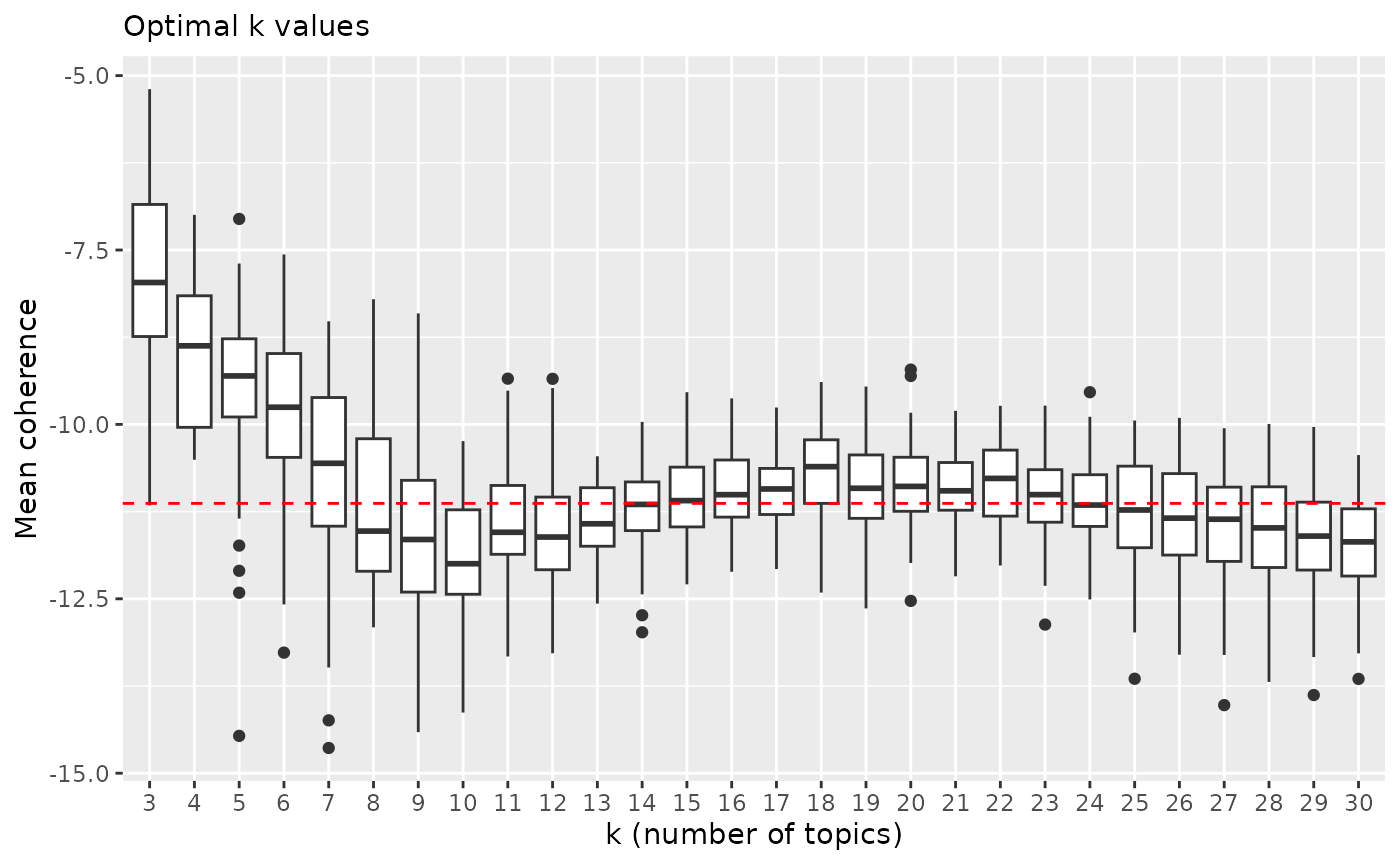
Above we can see that lowest quantile with K=18 is higher than any other from K 7 and above. Lower quantile of coherence score (horizontal dashed line) is even higher than for example highest quantile with K=10. There is some variation but to lesser degree than with k values below 10.
NOTE! Coherence scores can change even for smallest adjustments to pre processing pipeline. Make your mind on those first and stick to it.
Highest coherence values: 18
optimal_params <- lda_models |>
  filter(K %in% optimal_k) |>
  slice_max(mean_coherence, n = 5)
optimal_params
#> # A tibble: 5 × 3
#>       K       S mean_coherence
#>   <int>   <int>          <dbl>
#> 1    18 5883911          -9.39
#> 2    18 9596041          -9.55
#> 3    18 1001069          -9.59
#> 4    18 3146759          -9.77
#> 5    18 5745450          -9.79
Train models with optimal k and some different random seeds.
ptm <- proc.time()
selected_models <- optimal_params |>
  mutate(
    lda = future_map2(K, S, \(k, s) {
      LDA(dtm, k = k, control = list(seed = s))
    }, .options = furrr_options(seed = NULL))
  )
proc.time() - ptm
#>    user  system elapsed
#>   3.488   0.098 103.948
selected_models
#> # A tibble: 5 × 4
#>       K       S mean_coherence lda
#>   <int>   <int>          <dbl> <list>
#> 1    18 5883911          -9.39 <LDA_VEM>
#> 2    18 9596041          -9.55 <LDA_VEM>
#> 3    18 1001069          -9.59 <LDA_VEM>
#> 4    18 3146759          -9.77 <LDA_VEM>
#> 5    18 5745450          -9.79 <LDA_VEM>
Extract beta and theta matrices with probabilities for terms per topic and documents per topic repectively.
Note!
tidytext::tidy()uses term gamma-matrix while in the research field term theta-matrix is used to describe probability distribution of topics per document. Here we rename gamma as theta. Do not get confused if at some point you come around with gamma instead of theta.
selected_models <- selected_models |>
  mutate(
    # Beta matrix
    beta = map(
      lda, \(x) tidy(x, matrix = "beta")
    ),
    # Theta matrix (gamma)
    theta = map(
      lda, \(x) {
        tidy(x, matrix = "gamma") |>
          rename(theta = gamma)
      }
    )
  )
selected_models
#> # A tibble: 5 × 6
#>       K       S mean_coherence lda       beta                  theta
#>   <int>   <int>          <dbl> <list>    <list>                <list>
#> 1    18 5883911          -9.39 <LDA_VEM> <tibble [54,684 × 3]> <tibble>
#> 2    18 9596041          -9.55 <LDA_VEM> <tibble [54,684 × 3]> <tibble>
#> 3    18 1001069          -9.59 <LDA_VEM> <tibble [54,684 × 3]> <tibble>
#> 4    18 3146759          -9.77 <LDA_VEM> <tibble [54,684 × 3]> <tibble>
#> 5    18 5745450          -9.79 <LDA_VEM> <tibble [54,684 × 3]> <tibble>
Let’s try to calculate how much there is similarity in topics between different models. Similarity of certain topics between different models could indicate more reliable topics.
TODO: Set probabilities of all but the top 10-40 terms to zero and calculate cosine similarity between all topic pairs.
# selected_models <- selected_models |> filter(K==5)
selected_models <- selected_models |> mutate(model_id = paste0(K, "_", S))
idx <- combn(unique(selected_models$model_id), 2)  # Unique pairs of K

beta <- selected_models |> select(K, model_id, beta)

topic_pairs <- list()
for (i in 1:ncol(idx)) {
  sel <- beta |> filter(model_id %in% idx[, i])  # Two rows at a time

  # Combine pair of rows to same row
  topic_pairs[[i]] <- tibble_row(
    K1 = sel[[1,"K"]], model1 = sel[[1,"model_id"]], beta1 = sel[[1,"beta"]],
    K2 = sel[[2,"K"]], model2 = sel[[2,"model_id"]], beta2 = sel[[2,"beta"]]
    )

}
topic_pairs <- bind_rows(topic_pairs)

topic_pairs <- topic_pairs |>
  mutate(

    topics1 = map(beta1, \(b1) {
      b1 |>
        pivot_wider(values_from = beta, names_from = topic) |>
        select(-term)
    }),

    topics2 = map(beta2, \(b2) {
      b2 |>
        pivot_wider(values_from = beta, names_from = topic) |>
        select(-term)
    }),

    r = map2(topics1, topics2, \(x1, x2) {
      cor(x1, x2)
    })#,

    # cossim = map2(topics1, topics2, \(x1, x2) {
    #   cosine(x1, x2)
    # })
  )
topic_pairs
#> # A tibble: 10 × 9
#>       K1 model1     beta1       K2 model2    beta2    topics1  topics2  r
#>    <int> <chr>      <list>   <int> <chr>     <list>   <list>   <list>   <list>
#>  1    18 18_5883911 <tibble>    18 18_95960… <tibble> <tibble> <tibble> <dbl[…]>
#>  2    18 18_5883911 <tibble>    18 18_10010… <tibble> <tibble> <tibble> <dbl[…]>
#>  3    18 18_5883911 <tibble>    18 18_31467… <tibble> <tibble> <tibble> <dbl[…]>
#>  4    18 18_5883911 <tibble>    18 18_57454… <tibble> <tibble> <tibble> <dbl[…]>
#>  5    18 18_9596041 <tibble>    18 18_10010… <tibble> <tibble> <tibble> <dbl[…]>
#>  6    18 18_9596041 <tibble>    18 18_31467… <tibble> <tibble> <tibble> <dbl[…]>
#>  7    18 18_9596041 <tibble>    18 18_57454… <tibble> <tibble> <tibble> <dbl[…]>
#>  8    18 18_1001069 <tibble>    18 18_31467… <tibble> <tibble> <tibble> <dbl[…]>
#>  9    18 18_1001069 <tibble>    18 18_57454… <tibble> <tibble> <tibble> <dbl[…]>
#> 10    18 18_3146759 <tibble>    18 18_57454… <tibble> <tibble> <tibble> <dbl[…]>
topic_pairs |> select(K1, K2, r) |>
  mutate(similarity = map(r, \(x) {
    x |>
      as_tibble(rownames = "topic1") |>
      pivot_longer(!topic1, names_to = "topic2", values_to = "r") |>
      summarise(similarity = sum(r > 0.9)/n(), .by = topic1)  # Threshold 0.9 for similarity. Reasonable?
  })) |>
  select(-r) |>
  unnest(similarity) |>
  summarise(mean_similarity = mean(similarity), .by = c(K1, topic1)) |>
  mutate(topic1 = as.factor(as.integer(topic1)),
         mean_similarity_by_ntopics = ((mean_similarity*K1)/(1/optimal_k))/optimal_k) |>  # TODO: similarity depends somehow on number of topics
  ggplot() +
  geom_col(aes(x = topic1, y = mean_similarity_by_ntopics)) +
  # geom_hline(yintercept = 1/optimal_k,linetype='dashed', color=c('red')) +
  facet_grid(~K1, scales = "free_x")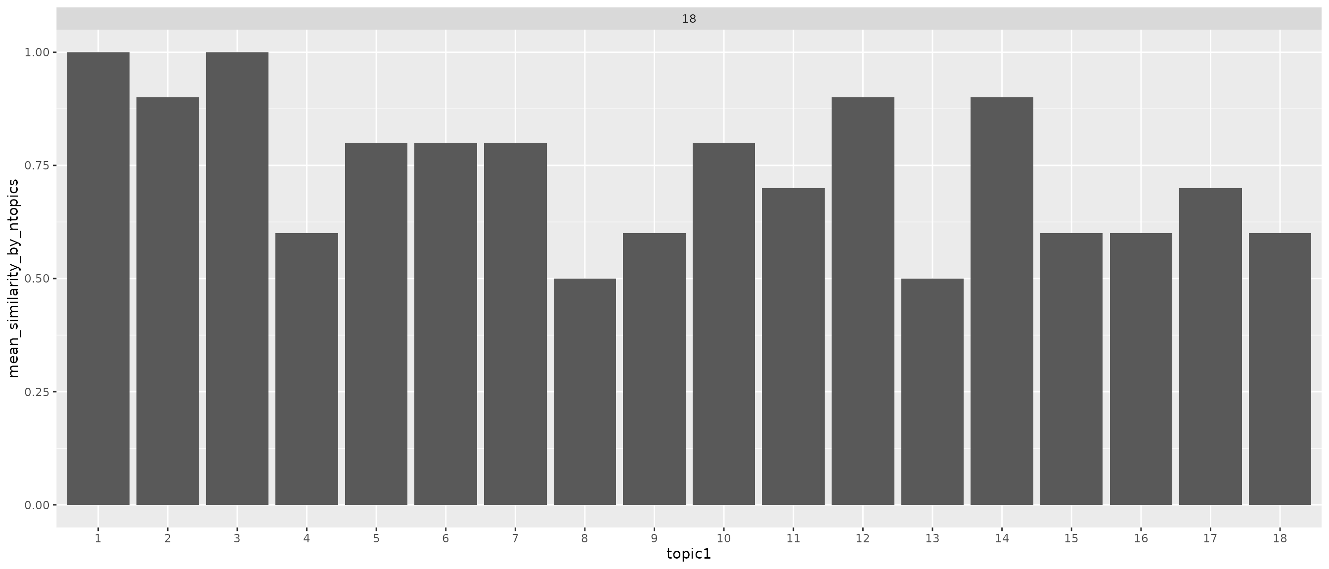
Above we calculated correlation between topics of one model and another model for all model topic pairs. Threshold for similarity was set to more than 0.9. Expected value if there is one matching topic for every model is 1 divided by number of topics (red dashed line). Topics 1 and 3 seems to appear in all models. In other hand topics 8 and 13 seem to be rather unique between models. This should be calculated with all 50 different models with same k value to get a better picture of what’s going on.
TODO:
Set probabilities of all but 10-40 most probable terms to 0.
Calculate cosine similarity between all topic-model pairs.
Define similarity with threshold 0.5-0.7
Summarise total similarity of different topics.
# topic_congruence <- list()
# for (i in 1:nrow(topic_pairs)) {
#   topic_congruence[[i]] <- topic_pairs$r[[i]] |>
#   as_tibble(rownames = "model1") |>
#   pivot_longer(cols = !model1, names_to = "model2", values_to = "r") |>
#   ggplot(aes(x = model1, y = model2, fill = r, label = round(r, 2))) +
#   geom_tile(show.legend = FALSE) +
#   geom_text() +
#   scale_fill_gradient2(low = "blue", mid = "white", high = "red")
# }
# plot_grid(plotlist = topic_congruence)
This is old work!
Next parts look ugly but hopefully they work. We take a look at
correlation between topics from different models to see if different
models catch up same things.
# topic_congruence <- list()
# for (i in selected_models$K) {
#   topic_congruence[[paste0("model-", i)]] <- selected_models |>
#   select(K, beta) |>
#   unnest(beta) |>
#   filter(K==i) |>
#   pivot_wider(values_from = beta, names_from = topic) |>
#   select(-term, -K)
# }
# topic_congruence
Compare all possible pairs of models:
# combn(selected_models$K, 2)
# topic_congruence2 <- list()
# for (idx_col in 1:ncol(combn(selected_models$K, 2))) {
#   idx <- combn(selected_models$K, 2)[, idx_col]
#   correlation <- cor(topic_congruence[[paste0("model-", idx[1])]], topic_congruence[[paste0("model-", idx[2])]])
#   topic_congruence2[[paste0("model-", idx[1], "-", idx[2])]] <- correlation |>
#     as_tibble(rownames = "topic1") |>
#     pivot_longer(!topic1, names_to = "topic2", values_to = "r")
# }
# topic_congruence2 <- bind_rows(topic_congruence2, .id = "model-K")
# topic_congruence2
# topic_congruence2 |>
#   mutate(`model-K`= factor(`model-K`),
#          topic1 = factor(as.integer(topic1)),
#          topic2 = factor(as.integer(topic2)),
#          r = round(r, 2)) |>
#   ggplot(aes(x = topic1, y = topic2, fill = r, label = r)) +
#   geom_tile(show.legend = FALSE) +
#   geom_text() +
#   theme(axis.text.x = element_text(angle = 90)) +
#   labs(title = "Topic congruence between different models") +
#   scale_fill_viridis_c(option = "A") +
#   facet_wrap(~`model-K`, scales = "free", ncol = 2)
Here we choose the final model(s) by largest coherence score.
final_models <- selected_models |>
  slice_max(mean_coherence, n = 1, by = K)
# final_models <- selected_models
How common are different topics over all?
final_models |>
  select(K, theta) |>
  unnest(theta) |>
  mutate(topic = factor(as.integer(topic))) |>
  summarise(mean_theta = mean(theta),
            total_theta = sum(theta), .by = c(K, topic)) |>
  ggplot() +
  geom_col(aes(x = topic, y = total_theta)) +
  labs(title = "Topic prevalence") +
  facet_wrap(~K, scales = "free")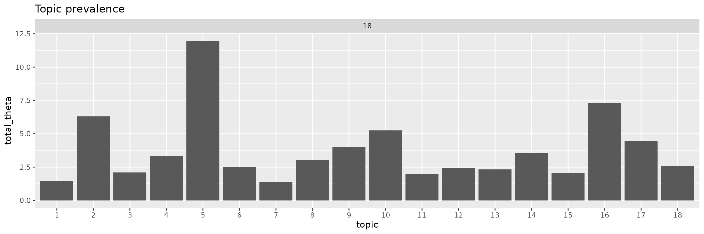
Topics 5 is most common by a large margin. Rarest are topics 1 and 7.
# final_models |>
#   select(K, theta) |>
#   unnest(theta) |>
#   ggplot(aes(x = theta, fill = K)) +
#   geom_histogram(binwidth = 0.1, show.legend = FALSE) +
#   labs(title = "Topic histograms") +
#   theme(axis.text.x = element_text(angle = 90)) +
#   facet_wrap(K~topic, scales = "free_y")
What is the share of the largest topic per document?
final_models |>
  select(K, theta) |>
  unnest(theta) |>
  slice_max(theta, n = 1, by = c(K, document)) |>
  mutate(topic = factor(as.integer(topic))) |>
  ggplot(aes(x = topic, y = theta, group = topic)) +
  geom_boxplot(show.legend = FALSE) +
  labs(title = "Distributions of largest topics per document") +
  facet_wrap(~K, scales = "free")
This figure gives a good idea of main topics which cover a large part or the whole of a document. Topics 1, 7, 12, 15 and 18 cover only large part of document.
# final_models |>
#   select(K, theta) |>
#   unnest(theta) |>
#   mutate(topic = factor(as.integer(topic))) |>
#   ggplot(aes(x = topic, y = theta, group = topic)) +
#   geom_boxplot(show.legend = FALSE) +
#   labs(title = "Topic distributions per document") +
#   facet_wrap(~K, scales = "free")
Here we take a look on topics and what they are. Remainder: most common topic was 5, rarest 1 and 7. Main topics were 1, 7, 12, 15 and 18.
final_models |>
  select(K, beta) |>
  unnest(beta) |>
  slice_max(beta, n = 25, by = c(K, topic)) |>
  group_by(K) |>
  add_count(term) |>
  ungroup() |>
  mutate(is_unique = n == 1,
         K = factor(K),
         topic = factor(topic),
         term = reorder_within(term, beta, topic)) |>
  ggplot(aes(x = beta, y = term, fill = K)) +
  geom_col(show.legend = FALSE) +
  labs(title = "25 terms with highest probability per topic") +
  scale_y_reordered() +
  facet_wrap(K ~ topic, scales = "free")
Same as above but only unique terms for topic.
final_models |>
  select(K, beta) |>
  unnest(beta) |>
  slice_max(beta, n = 25, by = c(K, topic)) |>
  group_by(K) |>
  add_count(term) |>
  ungroup() |>
  mutate(is_unique = n == 1,
         K = factor(K),
         topic = factor(topic),
         term = reorder_within(term, beta, topic)) |>
  filter(is_unique) |>
  ggplot(aes(x = beta, y = term, fill = K)) +
  geom_col(show.legend = FALSE) +
  labs(title = "25 terms with highest probability per topic") +
  scale_y_reordered() +
  facet_wrap(K ~ topic, scales = "free")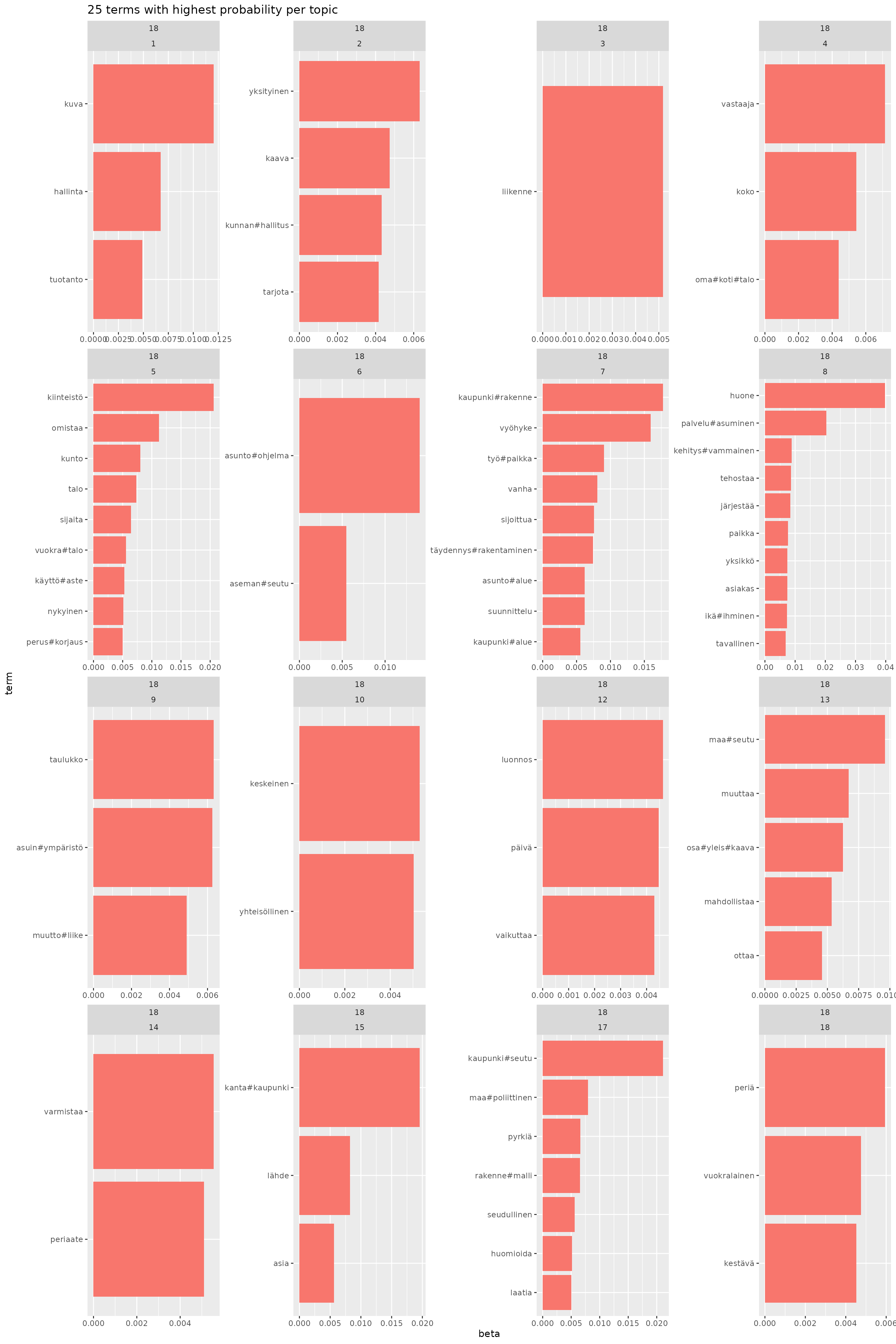
# for (i in unique(beta_matrix$model)) {
#   print(
#     beta_matrix |>
#       filter(model == i) |>
#       group_by(topic) |>
#       slice_max(beta, n = 25) |>
#       mutate(topic = as.factor(paste0("Topic_", topic))) |>
#       ggplot(aes(x = beta, y = reorder(term, beta), fill = topic)) +
#       geom_col(show.legend = FALSE) +
#       scale_fill_viridis_d(option = "A") +
#       facet_wrap(~topic, scales = "free") +
#       labs(title = "Top 25 terms by topic", subtitle = paste0("Model_", i), x = "Probability", y = "Term")
#   )
# }
# for (i in unique(beta_matrix$model)) {
#   print(
#     beta_matrix |>
#       filter(model == i) |>
#       group_by(topic) |>
#       slice_max(beta, n = 25) |>
#       mutate(topic = as.factor(paste0("Topic_", topic))) |>
#       ungroup() |>
#       add_count(term, name = "in_topics") |>
#       filter(in_topics == 1) |>
#       ggplot(aes(x = beta, y = reorder(term, beta), fill = topic)) +
#       geom_col(show.legend = FALSE) +
#       scale_fill_viridis_d(option = "A") +
#       facet_wrap(~topic, scales = "free", ncol = 2) +
#       labs(title = "Unique terms out of top 25 terms by topic", subtitle = paste0("Model_", i), x = "Probability", y = "Term")
#   )
# }
# doc_topics <- lapply(lda_models, function(x) {
#   x |>
#     tidytext::tidy(matrix = "gamma") |>
#     tidytext::cast_dfm(document, topic, gamma)
# })
# doc_topics
# join_y <- function(df) {
#   df |>
#     left_join(taantuvat, by = join_by("doc_id" == "kunta")) |>
#     filter(!is.na(luokka))
# }
# summarise_topics <- function(df, ...) {
#   df |>
#     mutate(topic = factor(as.integer(topic))) |>
#     summarise(...)
# }
# plot_topic_mean_prop <- function(df, ...) {
#   df |>
#     ggplot() +
#     geom_point(aes(...))
# }
# lapply(doc_topics, function(x) {
#   x |>
#     gather_topic_prob() |>
#     join_y() |>
#     summarise_topics(sum_prop = sum(prop), .by = c(luokka, topic)) |>
#     plot_topic_mean_prop(x = topic, y = sum_prop, colour = luokka)
# }
# )
# lapply(doc_topics, function(x) {
#   x |>
#     gather_topic_prob() |>
#     join_y() |>
#     summarise_topics(mean_prop = mean(prop), .by = c(luokka, topic)) |>
#     plot_topic_mean_prop(x = topic, y = mean_prop, colour = luokka)
# }
# )
# taantuvat |>
#   filter(kunta %in% unique(aspol$kunta)) |>
#   mutate(luokka = if_else(suht_muutos_2010_2022 > 0, "Kasvava", "Taantuva")) |>
#   count(luokka, sort = TRUE)
# purrr::imap(doc_topics, function(x, name) {
#   x |>
#     gather_topic_prob() |>
#     join_y() |>
#     select(doc_id, topic, prop, suht_muutos_2010_2022, luokka) |>
#     tidyr::pivot_wider(names_from = topic, values_from = prop) |>
#     rename_with(~ paste0("topic_", .x, recycle0 = TRUE), matches("^[0-9]+$")) |>
#     write.csv(paste0("topic_", name, ".csv"))
# })
# dat <- doc_topics$k_5 |>
#   gather_topic_prob() |>
#   join_y() |>
#   mutate(luokka = if_else(suht_muutos_2010_2022 > 0, "Kasvava", "Taantuva"),
#          topic = factor(as.integer(topic))) |>
#   select(topic, prop, luokka)
# dat
# for (i in seq_along(unique(dat$topic))) {
#   cat("Topic ", i)
#   print(
#     dat |> filter(topic == i) |>
#     ggplot() +
#     geom_boxplot(aes(x = luokka, y = prop)) +
#       labs(title = paste0("Topic ", i))
#     )
#   print(
#     dat |>
#       filter(topic == i) |>
#       kruskal.test(luokka ~ prop, data = _)
#   )
# }
# doc_topics$k_5 |>
#   gather_topic_prob() |>
#   join_y() |>
#   mutate(luokka = if_else(suht_muutos_2010_2022 > 0, "Kasvava", "Taantuva"),
#          topic = factor(as.integer(topic))) |>
#   summarise(topic_sum = sum(prop),
#             topic_mean = mean(prop),
#             .by = c(luokka, topic)) |>
#   kruskal.test(topic_sum ~ luokka)
# lapply(doc_topics, function(x) {
#   x |>
#     gather_topic_prob() |>
#     join_y() |>
#     mutate(luokka = if_else(suht_muutos_2010_2022 > 0, "Kasvava", "Taantuva"),
#            topic = factor(as.integer(topic))) |>
#     summarise(mean_prop = mean(prop), .by = c(luokka, topic)) |>
#     tidyr::pivot_wider(names_from = luokka, values_from = mean_prop) |>
#     mutate(diff = Kasvava-Taantuva) |>
#     ggplot() +
#     geom_point(aes(x = topic, y = diff)) +
#     ylim(-0.4, 0.4) +
#     geom_hline(yintercept = 0)
# })
# lapply(doc_topics, function(x) {
#   x |>
#     gather_topic_prob() |>
#     join_y() |>
#     mutate(luokka = if_else(suht_muutos_2010_2022 > 0, "Kasvava", "Taantuva"),
#            topic = factor(as.integer(topic))) |>
#     summarise(topic_sum = sum(prop),
#               topic_mean = mean(prop),
#               .by = c(luokka, topic)) |>
#     ggplot() +
#     geom_tile(aes(x = topic, y = luokka, fill = topic_sum)) +
#     scale_fill_viridis_c(option = "A")
# }
# )
# lapply(doc_topics, function(x) {
#   x |>
#     gather_topic_prob() |>
#     join_y() |>
#     mutate(luokka = if_else(suht_muutos_2010_2022 > 0, "Kasvava", "Taantuva"),
#            topic = factor(as.integer(topic))) |>
#     summarise(topic_sum = sum(prop),
#               topic_mean = mean(prop),
#               .by = c(luokka, topic)) |>
#     ggplot() +
#     geom_tile(aes(x = topic, y = luokka, fill = topic_mean)) +
#     scale_fill_viridis_c(option = "A")
# }
# )
# lapply(doc_topics, function(x) {
#   x |>
#     gather_topic_prob() |>
#     join_y() |>
#     mutate(luokka = if_else(suht_muutos_2010_2022 > 0, "Kasvava", "Taantuva"),
#            topic = factor(as.integer(topic))) |>
#     summarise(mean_prop = mean(prop), .by = c(luokka, topic)) |>
#     tidyr::pivot_wider(names_from = luokka, values_from = mean_prop) |>
#     mutate(diff = Kasvava-Taantuva) |>
#     tidyr::pivot_longer(Kasvava:Taantuva, names_to = "luokka", values_to = "prop") |>
#     ggplot() +
#     geom_tile(aes(x = topic, y = luokka, fill = diff)) +
#     scale_fill_distiller(palette = "Spectral")
# })
# titles <- aspol |>
#   group_by(kunta) |>
#   slice_head(n=10) |>
#   summarise(title = paste(FORM, collapse = " ")) |>
#   inner_join(taantuvat)
# titles
# titles_per_topics <- lapply(doc_topics, function(x) {
#   gather_topic_prob(x) |>
#     slice_max(order_by = prop, n = 1, by = doc_id) |>
#     left_join(titles, by = join_by("doc_id" == "kunta"))
#   })
# titles_per_topics
# titles_per_topics$k_5 |>
#   filter(topic==3) |>
#   select(doc_id, title)
# doc_topics$k_5 |> convert(to = "data.frame") |>
#   tidyr::pivot_longer(!doc_id, names_to = "topic", values_to = "prop") |>
#   left_join(taantuvat, by = join_by("doc_id" == "kunta")) |>
#   filter(!is.na(luokka)) |>
#   group_by(luokka, topic) |>
#   summarise(mean_prop = mean(prop)) |>
#   ggplot() +
#   geom_point(aes(x = topic, y = mean_prop, colour = luokka))
# doc_topics$k_5 |> convert(to = "data.frame") |>
#   tidyr::pivot_longer(!doc_id, names_to = "topic", values_to = "prop") |>
#   ggplot() +
#   geom_col(aes(x = prop, y = topic))